

Large enterprises often serve hundreds of thousands of users, which comes with massive computational demands. To keep business operations running smoothly and enhance customer experience, many companies are turning to deep learning models powered by machine learning (ML).
However, these models require significant computational resources during both training and inference. Training, in particular, involves running through large datasets dozens or even hundreds of times, which can heavily tax hardware and memory over time.
Running deep learning on edge devices — like mobile phones or other local hardware — is very different from training on a cloud-based GPU cluster. Edge training usually involves fine-tuning pre-trained models for just a few epochs. In contrast, on-device inference, where the model makes predictions locally, is increasingly common in modern applications.
While deep learning enables powerful applications, deploying these models on edge devices comes with its own set of challenges, from storage limits to energy constraints. Let's take a closer look.
CHALLENGES OF RUNNING NEURAL NETWORKS ON EDGE DEVICES
Running current neural networks on edge devices presents several constraints:
- Storage size: Most deep learning models take up 50 to 500 MB of space. While modern phones have plenty of storage, usually 32 to 512 GB, most people have many apps on their devices, and many apps use more than one neural network. All these models add up quickly. On top of that, app stores like Google Play and the Apple App Store limit the maximum size of an app, so keeping models small is essential.
- CPU utilization: A mobile phone’s CPU runs many apps at the same time and isn’t as powerful as a computer’s CPU. Running a neural network on the device requires a lot of computation, which can slow down your phone and make the user experience less smooth.
- Energy consumption: Since running a neural network makes the CPU work hard, it also drains more battery. The heavier the workload, the faster the phone uses up its energy, sometimes running out of charge in just a few hours.
Given these constraints, optimizing computational demand and compressing model weights is critical.
COMPRESSION AND OPTIMIZATION METHODS
In recent years, AI researchers have developed several methods to compress and optimize neural networks. Some focus on reducing time and computational efficiency, while others aim to shrink model size.
- Knowledge distillation: Transfers knowledge from a large, resource-intensive “teacher” model to a smaller “student” model. This produces compact models with comparable performance. However, it requires training from scratch, and results vary depending on the task.
- Weight sharing (quantization): Groups similar neurons into clusters, reducing the number of distinct weights. This can reduce model size by 10–15 times with minimal impact on performance.
- Pruning: Removes neurons, channels, or layers with low impact on the final output. This technique reduces both model size and inference time.
- Quantization: Reduces numerical precision of weights from 32 bits to 16, 8, or even 4 bits, leading to smaller models and faster inference.
- Binarization: An extreme form of quantization, where weights are reduced to just two bits. It offers high compression and speedup but can significantly reduce model accuracy if not used carefully.

EFFICIENT AI: YOUR DATA, BUT MORE EFFICIENT
Make your AI run faster, use less memory, and stay accurate — all while consuming less energy. Explore nowIMPLEMENTATIONS
To test these compression methods, we applied them to three CNN classifiers: MobileNetV2, ResNet50, and SqueezeNet1.1, using the ImageNet dataset for benchmarking.
PyTorch Quantization
PyTorch supports three quantization types: dynamic, static, and quantization aware training (QAT).
- Dynamic quantization: Weights are quantized ahead of time, while activations are quantized dynamically during inference. Currently, it supports only a few layers (fully connected, LSTM, and RNN), limiting its usefulness for CNNs or other NN architectures. During compressing CNN, only these certain layers will be quantized, which you can see from our results.
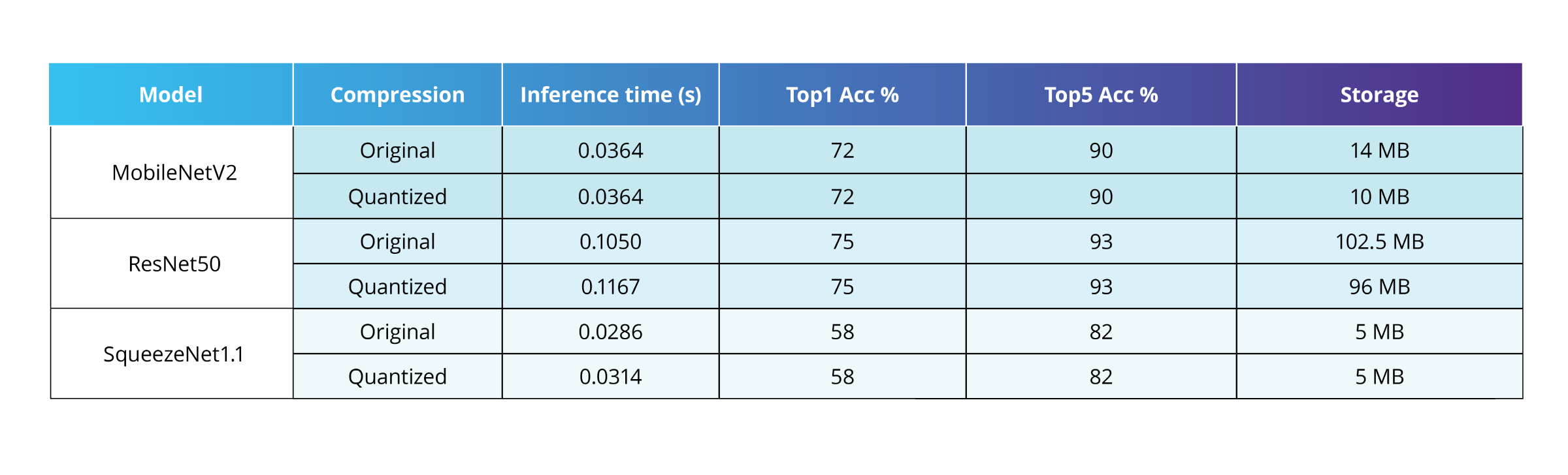
MobileNetV2 and ResNet50 both include a fully connected layer, which contributes to some reduction in model size after compression. In contrast, SqueezeNet1.1 does not show this effect because it lacks fully connected, LSTM, or RNN layers.
- Static quantization: Also known as post-training quantization, it quantizes weights ahead of time and includes a calibration step on a subset of data. This determines how activations are quantized during inference. With static quantization, we achieved 3–4× model compression and 1.2–3× inference speedup, depending on the NN architecture.
- Quantization aware training (QAT): During QAT, the model behaves as if weights and activations are quantized while computations are performed with floating-point values, which are rounded after each operation. QAT achieves the best accuracy compared to dynamic and static quantization but requires training from scratch.
PyTorch Pruning
In PyTorch, pruning can be done in two ways: local or global. With local pruning, neurons are removed based on the statistics of a single chosen layer. With global pruning, the decision is made using the statistics of the entire network.
In practice, pruning in PyTorch works by setting the weights and biases of selected neurons to zero. This means the model’s architecture doesn’t actually change, so you won’t see compression or speed improvements.
CoreML quantization
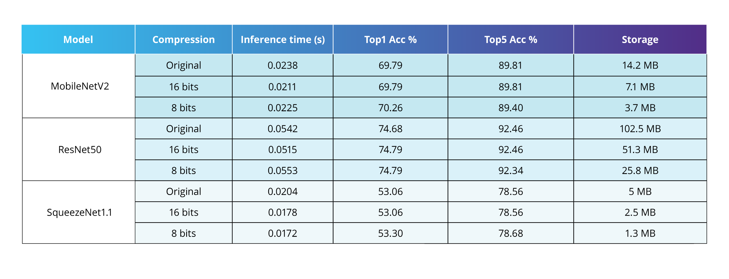
CoreML is Apple’s framework for running deep learning models on mobile devices. With Python’s coremltools package, you can easily apply quantization through a simple API. Model weights can be reduced from 16 bits to as low as 1 bit, with different modes available for 8–1 bit quantization. You can also choose which layers to quantize for more flexibility.
In our experiments, quantizing to 16 or 8 bits gave the same accuracy and inference speed, but reduced the model size in proportion to the number of bits.
Other toolkits for compression and optimization include TensorFlow Lite (quantization, pruning, weight sharing), Microsoft NNI (quantization, pruning), and IntelLabs Distiller (quantization, pruning, knowledge distillation).
CONCLUSION
Deep learning models bring enormous potential, but running them efficiently on mobile and edge devices requires careful optimization. Techniques like pruning, quantization, and model compression make it possible to balance performance with storage, speed, and energy limits.
SoftServe has deep expertise in tackling complex deep learning model challenges, including data engineering, ML, and production deployment for inference at scale. Get in touch with us to learn more.
Start a conversation with us