

Introduction

Machine learning (ML) can address modern upstream business and technical challenges, as well as bridge the gap between exploration data, science, IT, business stakeholders, and end-users.
In our recent webinar, “Machine learning for Exploration with Amazon SageMaker” SoftServe and AWS dove into how to quickly reach drill or no drill decisions from huge amount of seismic data, how to set up correct workflows in reservoir economics, and ultimately reduce the time to first oil production.
There are numerous ways ML can help automate your routine and manual interpretation steps. From navigating your seismic data and all exploration documents, to data enhancement and rapid processing of seismic and well-logs data.
Manual seismic data interpretation is time-consuming—taking weeks, months, or even longer. To accelerate processing, companies may require additional geoscientists which increases project costs.
In this white paper we will review, how to build an ML solution for seismic data interpretation and integrate it with your GEO tool of choice. In this case, we will use OpendTect.
We will explore the different aspects of this elaborate process, including:
- Data annotation and export for training
- Required data and annotations pre-processing
- Training and deploying a semantic segmentation model on Amazon SageMaker
- Evaluating the results and exporting them back to the GEO tool
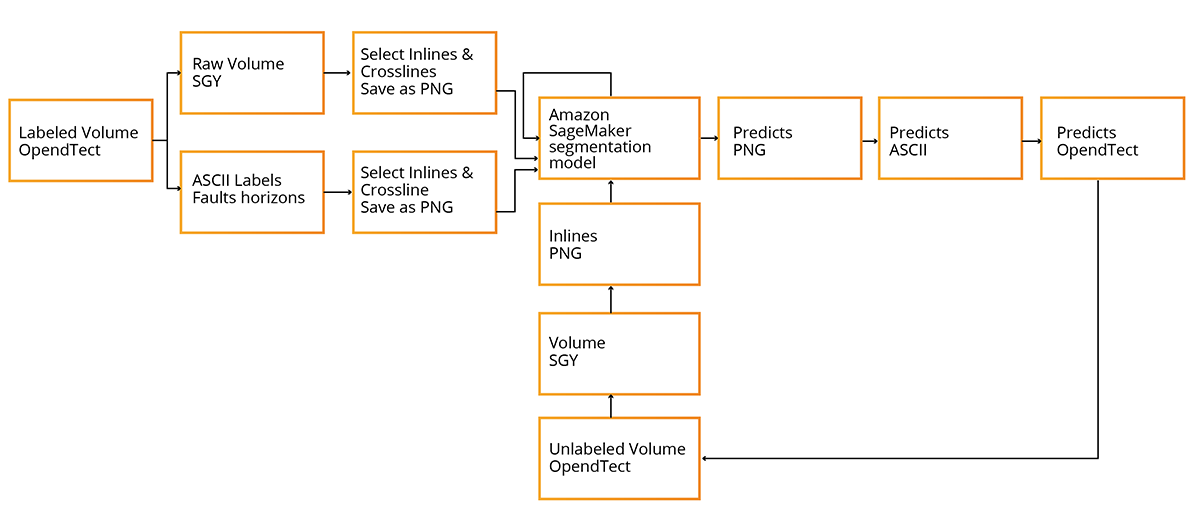
Here is the process flow we showed during the webinar.
Manual Interpretation
Seismic interpretation is the extraction of subsurface geologic information from seismic data. Manual seismic interpretation is a process in which geoscientists rely on their experience and knowledge, using various software and additional data, to choose the most likely interpretation from the many “valid” interpretations for each geological element that is analyzed.
For the purpose of this white paper we have interpreted three seismic volumes using OpendTect software and manually picked and annotated horizons in each.
Manual interpretation video episode from the webinar:
Data
Annotated data is a crucial aspect for training most of the ML models. For our train and validation set, we will use two volumes, Poseidon and Kerry. For the independent test set, we will use Parihaka. All of these data sets are publicly available.
Kerry and Parihaka are both 3D seismic volumes from New Zealand, off-shore. The Parihaka 3D survey comes from the Taranaki Basin, a full angle stack. The 3D volume is final anisotropic, Kirchhoff, prestack, time migrated. The Kerry 3D survey is also from the Taranaki Basin and is a prestack time migrated volume. The third seismic volume is from Australia, offshore. The Poseidon 3D survey is from the Australian NW shelf, Browse Basin, full stack, time migrated.
All three volumes were interpreted in OpendTect by an experienced geophysicist, and the main horizons were annotated.
This data in raw format may be downloaded from:
Poseidon 3D - https://terranubis.com/datainfo/NW-Shelf-Australia-Poseidon-3D
Kerry 3D - https://wiki.seg.org/wiki/Kerry-3D
Parihaka 3D - https://wiki.seg.org/wiki/Parihaka-3D#Download_data_clicking_links_or_command_line_wget
Problem Statement
In this white paper, we are going to train a binary semantic segmentation model on image representations of seismic volume in-lines.
In digital image processing and computer vision, image semantic segmentation is the process of partitioning a digital image into multiple segments. The goal of segmentation is to simplify and/or change the representation of an image into something that is more meaningful and easier to analyze.
The image below represents a binary semantic segmentation problem with two classes: plane and sky (background).

Processing a seismic volume as a set of 2D images (by cross-lines, in-lines, depth slices) is a common way of seismic data interpretation and has many advantages.
- It allows usage of a wide range of available segmentation model architectures out of the box
- It allows usage of pretrained models, thus reducing the amount of required labeled data
However, this approach also has some drawbacks.
- Predictions have to be interpolated and smoothed from in-line to in-line
- Model does not use contextual data from other in-lines and cross-lines (information from other dimensions)
Data Pre-processing
In-lines Extraction
The first step in working with the data, is reading the seismic volume and transforming it into a format consumable by the semantic segmentation model. Our main seismic data interpretation tool is OpendTect.
OpendTect is a complete open source seismic interpretation package, which is widely used in the industry and that can be downloaded at no cost from OpendTect. OpendTect contains all the tools needed for a 2D and/or 3D seismic interpretation: 2D and 3D pre- and post-stack, 2D and 3D visualization, horizon and fault trackers, attribute analysis and cross-plots, spectral decomposition, well tie, time-depth conversion, etc.
There are many seismic data formats, but, SEG-Y (SGY) is arguably the most widely used, and we will use it throughout the course of this white paper.
The SEG-Y file format is one of several standards developed by the Society of Exploration Geophysicists for storing geophysical data. It is an open standard, and is controlled by the SEG Technical Standards Committee, a non-profit organization.
Volumes converted to SGY format may be found at these links:
Poseidon: https://ml-for-seismic-data-interpretation.s3.amazonaws.com/SEG-Y/Poseidon_i1000-3600_x900-3200.sgy
Kerry: https://ml-for-seismic-data-interpretation.s3.amazonaws.com/SEG-Y/Kerry3e.sgy
Parihaka: https://ml-for-seismic-data-interpretation.s3.amazonaws.com/SEG-Y/Parihaka_PSTM_full-3D.sgy
Once we have the data in an SGY format, it’s time to begin in-lines extraction. We are going to use the Segyio library, https://github.com/equinor/segyio. Segyio is a small LGPL licensed C library for easy interaction with SEG-Y and Seismic Unix formatted seismic data, with language bindings for Python and Matlab.
The first thing is to read the volume.
volume = segyio.tools.cube(volume_location)
In this example ,we are going to use in-lines, so we need to transpose the volume so that in-lines are represented by the first diminution.
volume = volume.transpose((0, 2, 1))
In-lines are chosen for the simplicity of prototyping, however, for the production ready system it is important to extend the model to process cross-lines and depth-slices as well.
Now, we have a raw volume in a correct format, but we also need to remove the outliers and noise from the data. To do this, we will drop all the signal above the 99.5 and below the 0.5 percentiles. This could be done with the clip_normalize_cube function.
def clip_normalize_cube(cube, percentile=99.5):
    right = np.percentile(cube, percentile)
    left = np.percentile(cube, 100 - percentile)
    bound = np.max([np.abs(left), np.abs(right)])
    np.clip(cube, -bound, bound, cube)
    cube /= bound
    return cube
volume = clip_normalize_cube(volume)
So, the volume was transformed and basic outlier removal was done, but the values in the volume still float from –1 to 1.
Our goal is to export in-lines as set of grayscale images that are represented by unit values from 0 to 255. We therefore need to perform normalization and discretization.
volume = ((volume + 1) * 255 // 2)Once those steps are complete, we can iterate over the in-lines and save them as JPG or PNG images.
idx = starting_idx
for img in volume:
    plt.imsave(f'kerry/{str(idx}.png',
    img.astype(int) , cmap='gray')
    idx += 1
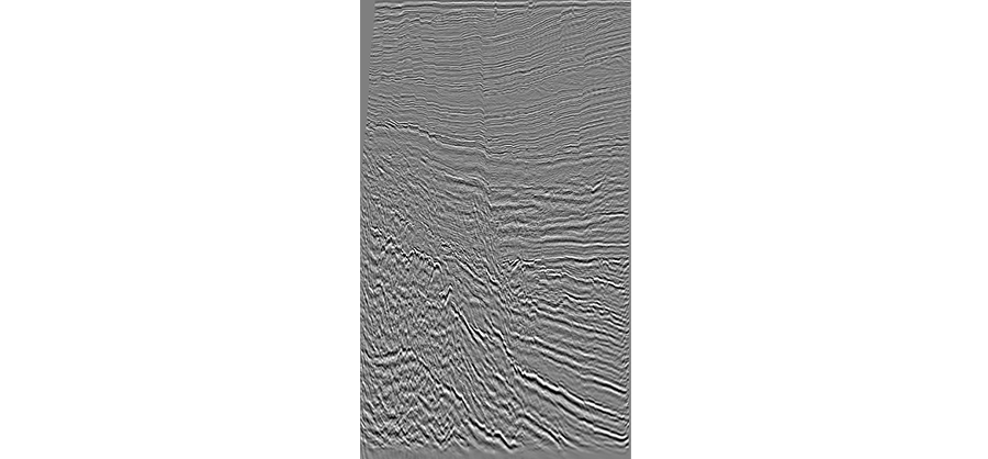
The resulting pictures should look similar to the one below. Note the shape will depend on the volume that you are processing, the current in-line is from the Kerry volume.
Annotations Extraction
As for the annotations, the best way to export them from OpendTect is ASCII format files, with the following structure:
Horizons – lines in the file represent 3D coordinates of the points defining the horizon line:
# "Inline"	"Crossline"	"Z"
# - - - - - - - - - -
"h_antique_01"	 	2601	4200	2306.90836906
"h_antique_01"		2601	4201	2306.35046959
"h_antique_01"		2601	4202	2305.92775345
"h_antique_01"		2602	4200	2306.85067177
"h_antique_01"		2602	4201	2306.48946762
"h_antique_01"		2602	4202	2305.98044395
"h_antique_01"		2602	4203	2305.44114113
"h_antique_01"		2602	4204	2304.49652672
Horizon annotation files may be accessed on S3 using the links below.
Poseidon: https://ml-for-seismic-data-interpretation.s3.amazonaws.com/Annotations/Poseidon_h_ix_bulk.dat
Kerry: https://ml-for-seismic-data-interpretation.s3.amazonaws.com/Annotations/Kerry_h_ix_bulk.dat
Parihaka: https://ml-for-seismic-data-interpretation.s3.amazonaws.com/Annotations/Parihaka_h_ix_bulk.dat
Our goal is to reconstruct a 3D volume, match it with our raw seismic data, and export all those as PNG masks for the semantic segmentation algorithm.
To achieve this, we are going to reconstruct an empty volume and populate it with non-zero values (e.g. 255) for each 3D point in the annotation file.
We begin by defining an empty array with the same shape as our seismic volume.
shape = (2601, 1326, 2301) # Poseidon volume shape horizons = np.zeros(shape, dtype=int)
Afterwards, we need to parse the annotation file and extract horizon coordinates from there.
horizons_dat = [i.strip().split() for i in open("Poseidon_h_ix_bulk.dat").readlines()]
Each volume has a set of hyperparameters, such as starting and ending in-line/cross-line and Z-step.
For example, Poseidon is a volume with a shape (2601, 1326, 2301), where in-lines are from 1000 to 3600, cross-lines 900 to 3100, Z with a step of 4.
Let’s define those parameters, as we need them to match the original seismic volume and our annotations.
starting_inline = 1000
starting_crossline = 900
z_step = 4
horizons_dat = [[int(i[1]) - starting_inline, int(i[2])- starting_crossline, round(float(i[3])/z_step)] for i in horizons_dat if not (i[1]=='"Inline"' or i[1]=='-')]
As a result, we will get an array of horizon coordinates.
[[2424, 1660, 267],
 [2424, 1661, 267],
 [2424, 1662, 267],
…
We could use those coordinates to populate the empty volume.
for h in horizons_dat:
    horizons[h[0]][h[2]][h[1]] = 255
As a result, we got a binary volume where horizons are represented by non-zero values and everything else is zero. Therefore, we could iterate again over in-lines in the annotation volume and save them as PNG images.
idx = 1000 #Starting In-line
for img in tqdm(horizons):
    img_name = f'masks/h/{idx}.png'
    plt.imsave(img_name, img.astype(int) , cmap='gray')
    idx += 1
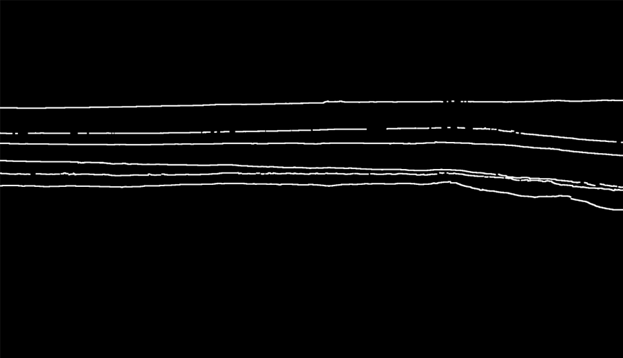
The resulting masks will be black and white and will look similar to the one below (for Poseidon volume).
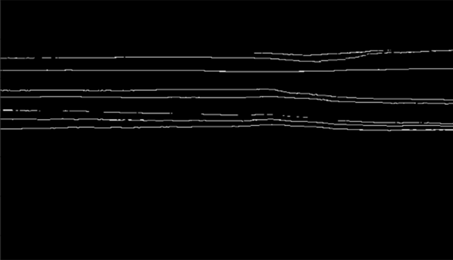
As we can see, horizons on those masks are annotated with 1px wide lines. However, such representation is poorly suitable for training the semantic segmentation model.
In our case, we have a binary semantic segmentation problem with two classes, horizon and background. Our horizon lines are extremely thin and we have a significant class imbalance towards the background. Additionally, in nature, horizons are represented by much wider segments on the seismic volume.
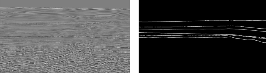
To reduce the impact of these problems, we will perform the dilation of the lines on the masks.
Dilation is a morphological operation used to enhance the features of an image. Dilation as a function requires two inputs – an image to be dilated and a two dimensional structuring element. Dilation has many applications, but is most commonly used to exaggerate features in an image that would otherwise be missed.
kernel_size = 3
mask = mask.filter(ImageFilter.MaxFilter(kernel_size))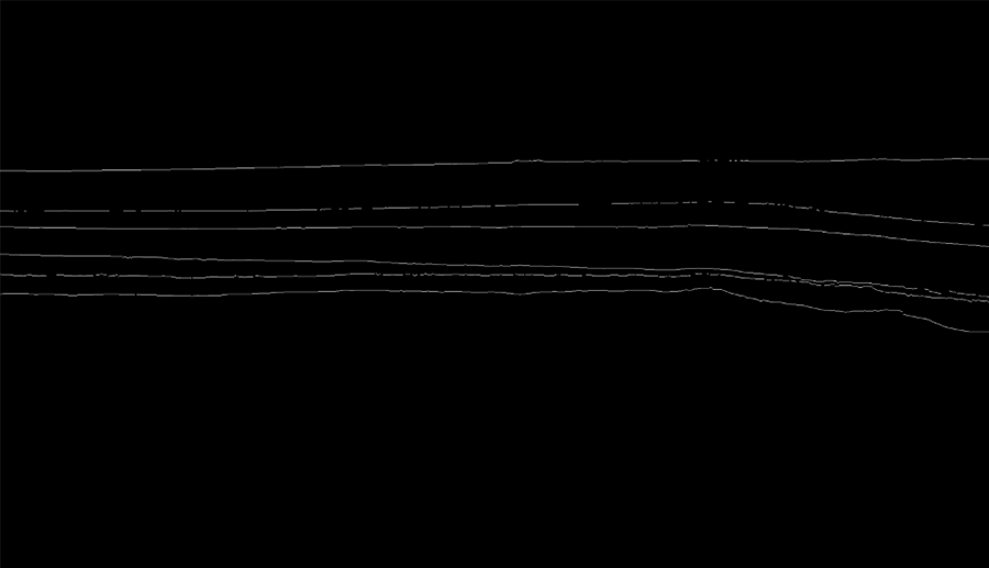
after
Validation/Test Set Split
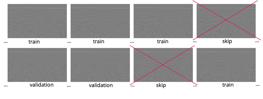
One of the common challenges and pitfalls in training seismic data interpretation models is the correct selection of train, validation, and test sets. The biggest problem is the correlation in the data. By nature, all the in-lines, cross-lines or z-slices are highly correlated, and the closer they are the higher the degree of correlation.
The presence of the highly correlated data in the train and validation sets will usually have a negative impact on model convergence and lead to the overfitting towards train data. If we split train and validation randomly, there’s a high chance that neighboring in-lines will appear in train and validation, which is exactly what we are trying to avoid.
On the other hand, if we split the volume into two parts, our train and validation might not follow the same distribution and may differ significantly.
Therefore, we need to divide each volume into multiple batches and skip chunks of data between train and validation. With this train-validation split, we minimize the correlation between sets and assure they both fully represent the volume.
Model Design and Train
While the data preprocessing steps could be done on local machine or using Amazon SageMaker Notebook Instances, it is useful to apply the capabilities of Amazon SageMaker for model training and deployment.
Amazon SageMaker is a fully managed service that provides every developer and data scientist with the ability to build, train, and deploy ML models quickly. SageMaker removes the heavy lifting from each step of the ML process to make it easier to develop high quality models.
Setting up SageMaker is an easy and smooth process that requires just a few clicks. We are using Amazon SageMaker Studio for data pre-processing, model training, and deployment.
In this case, we are using the Bring Your Own Script paradigm and fitting the data with an Apache MXNet framework. This approach allows us to use the default MXNet container and provides the code that defines the training. For an example, see Training and Hosting SageMaker Models Using the Apache MXNet Module API on GitHub.
Dataset and Data Loader
After the previous data processing steps, we now have a set of grayscale images and corresponding masks for each train, validation and test set.
It’s important to structure the dataset in a format expected by your dataset class. In our case, we are using default for the built-in semantic segmentation task dataset structure.
s3://bucket_name
    |- train
                 |
                 | - 0000.jpg
                 | - coffee.jpg
    |- validation
                 |
                 | - 00a0.jpg
                 | - bananna.jpg
    |- train_annotation
                 |
                 | - 0000.png
                 | - coffee.png
    |- validation_annotation
                 |
                 | - 00a0.png
                 | - bananna.png
    |- label_map
                 | - train_label_map.json
                 | - validation_label_map.json
For more information on the input data suggestions and limitations, please refer to https://docs.aws.amazon.com/sagemaker/latest/dg/semantic-segmentation.html
As all the preprocessing steps require significant time and resources, you could download an already constructed train-validation dataset here https://ml-for-seismic-data-interpretation.s3.amazonaws.com/dataset/train-val.zip
The test set data can be downloaded from the S3 bucket https://ml-for-seismic-data-interpretation.s3.amazonaws.com/dataset/test.zip
Unzip the archive and place the content on your S3 bucket for training.
The expected folder structure and all the image/mask preprocessing is defined by the dataset class. As we mentioned previously, with the Bring Your Own Script paradigm, it’s part of our responsibility to define the training helper classes.
Training Step
In our training, we are going to use the Bring Your Own Script paradigm and fit the data with a U-Net network written in Apache MXNet.
U-Net – Introduced in the paper U-Net: Convolutional Networks for Biomedical Image Segmentation, this network was originally used for medical-imaging use cases but has since proven to be reliable in generic segmentation domains. Due to its architectural and conceptual simplicity, it’s often used as a baseline.
MXNet - A truly open source deep learning framework suited for flexible research prototyping and production.
We are starting by importing the SageMaker and MXNet and defining role and session, which we will need over the whole course of training.
A session object provides convenience methods within the context of Amazon SageMaker and our own account. An Amazon SageMaker role ARN is used to delegate permissions to the training and hosting service. We need this so that these services can access the Amazon S3 buckets where our data and model are stored.
import sagemaker
import mxnet as mx
from sagemaker import get_execution_role
from sagemaker.mxnet import MXNet
sagemaker_session = sagemaker.Session()
role = get_execution_role()
After the imports, we create the data loader, which will be responsible for fetching the dataset from S3.
train_s3 = sagemaker.s3_input(s3_data='s3://aws-seismic-dataset/train-val', distribution='FullyReplicated')Having the s3_input defined, we can create an estimator object that handles end-to-end training and deployment tasks.
seismic_unet_job = 'Seismic-unet-job-' + \
    time.strftime("%Y-%m-%d-%H-%M-%S", time.gmtime())

seismic_estimator = MXNet(entry_point='seismic.py',
                  base_job_name=seismic_unet_job,
                  role=role,
                  py_version="py3",
                  framework_version="1.6.0",
                  train_instance_count=1,
                  train_instance_type='ml.p3.2xlarge',
                  hyperparameters={
                      'learning_rate': 0.003,
                      'batch_size': 2,
                      'epochs': 5
                     })
To test whether our model is training correctly, we are going to train it for just 5 epochs with a small batch_size on one train instance. Once we assure that model converges, we could relaunch the training for more epochs and with more resources.
We are using a dice-coefficient-based loss function.
def avg_dice_coef_loss(y_true, y_pred):
    intersection = mx.sym.sum(y_true * y_pred, axis=(2, 3))
    numerator = 2. * intersection
    denominator = mx.sym.broadcast_add
(mx.sym.sum(y_true, axis=(2, 3)),
mx.sym.sum(y_pred, axis=(2, 3)))
    scores = 1 - mx.sym.broadcast_div(numerator + 1.,
 denominator + 1.)
   return mx.sym.mean(scores)
Please note, it is recommended to test your scripts before launching the training on Amazon SageMaker Training Instances, as you may end up paying for setting up the instance each time before a bug or error is caught.
Local testing requires setting up MXNet Docker container locally, for more details, please refer to https://aws.amazon.com/blogs/machine-learning/use-the-amazon-sagemaker-local-mode-to-train-on-your-notebook-instance/
Once the setup is complete, local training could be enabled by setting train_instance_type parameter to local.
train_instance_type = ‘local’
To start the training, we are fitting the estimator with the train and validation datasets.
seismic_estimator.fit({'train': train_s3})
We have chosen the basic hyperparameters for the model training to test that it converges, although better performance could be reached with hyperparameters optimization.
Hyperparameters tuning is a complex and elaborate process and you could use automatic model tuning in Amazon SageMaker to launch hyperparameter tuning jobs that optimize on a given metric or metrics using Bayesian optimization.
As we use the MXNet framework version 1.6.0, seismic.py must be called as a standalone script and contain the functions ‘model_fn’, ‘transform_fn’ for hosting.
See https://sagemaker.readthedocs.io/en/stable/frameworks/mxnet/using_mxnet.html for details.
Please note, seismic.py should be uploaded to the root folder alongside the Jupyter notebook.
def transform_fn(net, data, input_content_type,
 output_content_type):
    """
    Transform a request using the Gluon model.
    Called once per request.

    :param net: The Gluon model.
    :param data: The request payload.
    :param input_content_type: The request content type.
    :param output_content_type: The (desired)
    response content type.
    :return: response payload and content type.
    """
    # we can use content types to vary input/output
    handling, but
    # here we just assume json for both
    try:
        input_data = json.loads(data)
        nda = mx.nd.array(input_data)
        nda *= 1.0/nda.max()
        output = net(nda)
        im =np.array(Image.fromarray((output.asnumpy()[0][0]*
 255).astype('uint8'), mode='L'))
        response_body = json.dumps(im.tolist())
    except Exception as e:
        logging.error(str(e))
        return  json.dumps([1,2]), output_content_type
    return response_body, output_content_type
Model Deployment and Testing
We can now deploy the trained model to serve inference requests. For this we are going to create a new endpoint and simply deploy the model there.
seismic_endpoint = 'Seismic-unet-endpoint-webinar'
seismic_predictor = seismic_estimator.deploy(instance_type='ml.c5.xlarge', initial_instance_count=1,
endpoint_name=seismic_endpoint)
It will take a few minutes to deploy the endpoint, but as soon as it’s done we could send new in-lines for the model interpretation.
The images will require basic preprocessing before sending.
response = seismic_predictor.predict(image)
img_out = np.array(response)
output =np.array(Image.fromarray(img_out.astype('uint8'),
mode='P').resize(( IM_WIDTH, IM_HEIGHT) ))
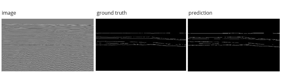
Below are the sample results on the validation set.
image ground truth prediction
Once model validation is finished, it’s important to delete the endpoint, as billing is done per hours it is deployed.
seismic_predictor.delete_endpoint()
Results Export for Further Interpretation
After the model training and deployment are complete, our model is ready to process new data and generate new insights.
However, our model still processes 2D in-lines, which are uncomfortable for further interpretation and cannot be exported back to OpendTect. We therefore need to postprocess the model output and convert it to the format readable by seismic interpretation tools.
We originally got our annotations in the format of structured file.
# "Inline"	"Crossline"	"Z"
# - - - - - - - - - -
"h_antique_01"	 	2601	4200	2306.90836906
"h_antique_01"		2601	4201	2306.35046959
"h_antique_01"		2601	4202	2305.92775345
We now need to process our predictions and save in the same format of 3D coordinates. This could be achieved through a multistep approach and application of various conventional computer vision algorithms.
Firstly, in the same way we performed dilation if the masks to make them wider, we need to transform the predictions back to 1px wide lines. This is achieved by applying skeletonization.
Skeletonization is a process for reducing foreground regions in a binary image to a skeletal remnant that largely preserves the extent and connectivity of the original region while throwing away most of the original foreground pixels.
We are using the skeletonize function from the skimage library https://scikit-image.org/docs/stable/auto_examples/edges/plot_skeleton.html

After skeletonization, we have a binary mask with all the horizons annotated as 1px wide lines.
These in-lines could already be exported to binary SEG-Y file for some of the seismic instruments. However, we want to go one step further and perform basic separation of the horizons, or their components. The easiest way is to identify all the separate line segments on the prediction mask and then merge them into horizons.
To separate line segments, we are using connected components identification algorithms.
For more details, please refer to http://scipy-lectures.org/packages/scikit-image/auto_examples/plot_labels.html
When the separate segments are identified and labeled, we could iterate over the in-lines and use 2D coordinates of the horizons to reconstruct the original 3D coordinates in the volume and save them in the original annotations format.
# "Inline"	"Crossline"	"Z"
# - - - - - - - - - -
"h_1000_1"	1000	900	1576
"h_1000_1"	1000	900	1580
"h_1000_1"	1000	900	1584
"h_1000_1"	1000	901	1576
"h_1000_1"	1000	901	1580
Results Evaluation and Active Learning
After model predictions are exported back to OpendTect (or any other interpretation software), the results can be viewed and validated for consistency in conventional software that is used by seismic interpreters (geoscientists) all over the world (Petrel, Kingdom). The integration with conventional software makes it possible to use the Active Learning Cycle, repeatable cycles during which a seismic 3D survey is split to separate volumes and one of them is manually interpreted and then used as the training and validation dataset for the mode.
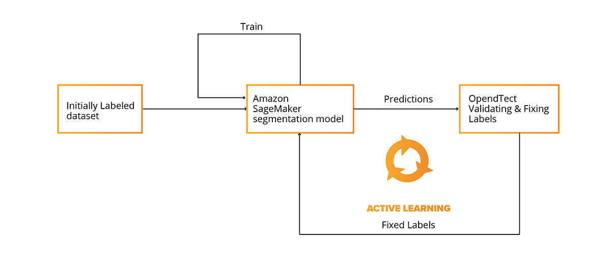
The trained model is then used to interpret the next volume, and afterwards is checked for consistency and fixed by an interpreter, if needed. For the next cycle, two interpreted volumes are already used for training and validation. This cycle can be repeated multiple times to increase the quality of model predictions and ultimately decrease time and automate structural interpretation.
The Active Learning Cycle makes it possible to create a seismic interpretation model without large scale prior preparation and seismic interpretation activities. The model can be trained during the normal interpretation workflow.
Active Learning video episode from the webinar:
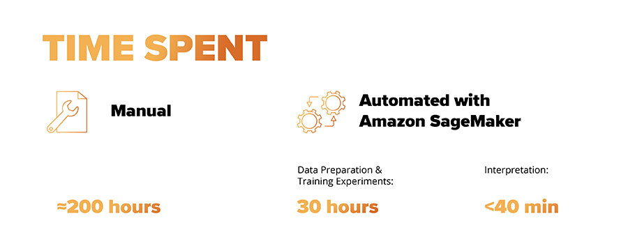
Summary
Below is a summary of the time spent automating horizons detection vs manual interpretation of the same data.
In this white paper, we explained how ML techniques can quickly add value to your existing business workflows or products as a geoscience service provider.
Thanks to advanced cloud technologies such as AWS and Amazon SageMaker, a typical engagement for such projects can be reduced from years down to months, or even weeks. These platforms can help mitigate risks around early experimental process and deliver rapid results from proven business concepts with minimal risk and initial commitment from clients.
SoftServe is ready to demonstrate how an online ideation workshop can be delivered as a first step to kick off true automation of seismic and well log data processing and optimization of other geophysical workflows for your business. Contact us today to get started.
References:
Full data preprocessing, model training and deployment code, can be found here
https://github.com/oilngas/ml-for-seismic-data-interpretation
https://docs.aws.amazon.com/sagemaker/latest/dg/semantic-segmentation.html/