

No one can whistle a symphony. It takes a whole orchestra to play it.
Collaboration is one of the most notable characteristics of mankind’s ability to overcome obstacles. It allows the whole to become greater than the sum of its parts.
Another characteristic, which becomes more and more important these days, is the ability to automate routines to free up mental resources for creative activities.
Collaboration is possible through communication, and automation is a prerogative of computers. Modern computers are very powerful but, much like a single human, the performance of a single computer is limited. Multiple computers have to collaborate to step beyond their individual limits. Thus, computers need to communicate too.
Communication is a complex activity which requires multiple overheads. One of these is SerDe — Serialization and Deserialization of messages — the process of converting a structured message into a format that can be used for the serial transmission of data over a medium and restoring it back.
Goals
This article observes and compares a set of popular serialization formats which can be used for the transportation and processing of big batches of structured data (hundreds of thousands of records) in the Python programming language. Its goal is to share the results and experience of examining the pros and cons of the following formats:
- CSV
- JSON
- JSON Lines
- msgpack
- Avro
- Protobuf
- Cap’n Proto
This article will help you to decide which format best fits your needs.
Something to think about
Always keep in mind that being a software engineer and operating almost exclusively with non-materialistic entities like ideas doesn’t mean you shouldn’t think about the impact of your ideas on materialistic world. In fact, you must. Especially today, when a simple software solution can easily propagate and scale around the globe. And with respect to nature, dear readers, please make sure your solutions are optimal and don’t waste energy and materials. The selection of a proper serialization format firmly relates to this.
Comparison apparatus
To compare several entities with each other, a list of criteria must be defined. In this article, we will use many criteria. To make it easier to comprehend, they are split into three groups: primary, secondary, and extra.
Primary criteria group
The primary group includes the most important criteria, which relate to resource usage:
- CPU consumption: measured by execution time;
- Main memory consumption: measured by resident set size (RSS);
- External memory consumption: measured by the size of the data that is going to be transferred and may be buffered to disc. This includes both compressed (tar.gz) and non-compressed data.
Secondary criteria group
Next, the secondary group includes criteria related to data type detection and validation:
- Supported set of data types;
- Available level of validation;
- Versioning.
Extra criteria group
Finally, the extra group defines criteria which might be useful, but not as critical as the previous group:
- Support of empty (optional) values;
- Ability to process batches of data as streams;
- Restrictions for format of field names;
- Steepening the learning curve/how hard it can be to start using it;
- Human-orientation (the ability to be able to be easily comprehended by humans);
- Computer-orientation (the ability to perform actions in an optimal way).
Test environment
A primary group of defined criteria requires us to examine the consumption of fundamental resources: time and space. This requirement will be satisfied by empirical research, as several measurements must be taken for each selected format of serialization. Of course, the results of the measurements depend on which environment they are taken from and whether it’s hardware or software.
Though we’re going to end up with a comparison of selected criteria using relative numbers (percent), absolute values must also be provided so that measurements can be repeated and compared. A list below describes a system configuration, which was used to perform tests:
- GYGABYTE GA-Z170-D3H motherboard (with Intel Z170 chipset);
- Intel Core i7–6700 CPU (4 physical cores, 8 virtual cores provided by hyper-threading, 3.40GHz);
- 32 Gb of DDR4 RAM (2x Kingston KHX2666C15/16GX, 2133 MHz);
- SSD 850 EVO SATA III (540MB/s seq. read, 520MB/s seq. write);
- 64-bit GNU/Linux kernel (4.8.0–58-generic, elementary OS 0.4.1 Loki);
- Python 3.4.5 (default, Jul 15 2016).
Test data set
As it was stated in the “Goal” section, we are interested in processing big batches of structured data, which have different data types: dates, strings, integers, floats and nulls, etc. So, before starting any measurements, a test data set must be prepared.
For this article we are going to take Airline On-Time Performance Data provided by the Bureau Of Transportation Statistics. We will use an exported data set which includes data from all US regions for January 2017 (data can be fetched from here).
Our data set includes 450,017 records with following fields (see glossary):
┌────────────────────────────────┐
│ Table 1 — Data field types     │
├───────────────────────┬────────┤
│         Name          │  Type  │
├───────────────────────┼────────┤
│ FL_DATE               │ Date   │
│ AIRLINE_ID            │ UInt32 │
│ CARRIER               │ String │
│ TAIL_NUM              │ String │
│ FL_NUM                │ UInt32 │
│ ORIGIN_AIRPORT_ID     │ UInt32 │
│ ORIGIN_AIRPORT_SEQ_ID │ UInt32 │
│ ORIGIN_CITY_MARKET_ID │ UInt32 │
│ ORIGIN                │ String │
│ ORIGIN_CITY_NAME      │ String │
│ ORIGIN_STATE_ABR      │ String │
│ ORIGIN_STATE_FIPS     │ UInt32 │
│ ORIGIN_STATE_NM       │ String │
│ ORIGIN_WAC            │ UInt32 │
│ DEST_AIRPORT_ID       │ UInt32 │
│ DEST_AIRPORT_SEQ_ID   │ UInt32 │
│ DEST_CITY_MARKET_ID   │ UInt32 │
│ DEST                  │ String │
│ DEST_CITY_NAME        │ String │
│ DEST_STATE_ABR        │ String │
│ DEST_STATE_FIPS       │ UInt32 │
│ DEST_STATE_NM         │ String │
│ DEST_WAC              │ UInt32 │
│ DEP_DELAY             │ Float  │
│ TAXI_OUT              │ Float  │
│ WHEELS_OFF            │ Float  │
│ WHEELS_ON             │ Float  │
│ TAXI_IN               │ Float  │
│ ARR_DELAY             │ Float  │
│ AIR_TIME              │ Float  │
│ DISTANCE              │ Float  │
└───────────────────────┴────────┘
Fetched data is represented by a dynamically generated CSV file. Unfortunately, raw data are not suitable for us as-is and source file needs to be a bit normalized.
First of all, we need to strip away trailing commas at the end of each line:
sed -i 's/,$//g' source.csv
Next, we need to quote dates, so they will comply format of strings:
perl -pi -e 's/^(\d{4}-\d{2}-\d{2}),/"\1",/g' source.csv
Now we have a ready-to-use data set with the following attributes:
┌──────────────────────────────────┐
│ Table 2 — Source data attributes │
├────────────────────────┬─────────┤
│        Attribute       │  Value  │
├────────────────────────┼─────────┤
│ Number of records, #   │ 450'017 │
│ Uncompressed size, MiB │    95.3 │
│ Compressed size,   MiB │    13.1 │
└────────────────────────┴─────────┘
Measurement approach
We need to run several tests to measure attributes for the primary criteria group. The test logic is the same for all serialization formats being tested:
- Load data from source CSV with automatic type detection.
- Save that data multiple times using target serializer and measure average run time and RSS. Each test runs in a separate process and makes writes to a separate temporary file.
- Save a single permanent file.
- Load serialized file multiple times using target deserializer and measure average run time and RSS. Each test runs in a separate process.
Multiple tests for a single serializer are run in parallel to save time. This is achieved by using concurrent.futures.ProcessPoolExecutor with number of max parallel workers equal to a number of virtual CPU cores (8 cores for described environment). The process pool is recreated after all subprocesses execute 1 test run. This is done to avoid memory caching. The number of tests per serializer is equal to twice the size of the pool, so there are 16 separate tests which are executed in 2 sequential batches, containing 8 tests in each.
The evaluation of measurement errors isn’t done, though measurements provide enough accuracy for comparison even including statistical errors.
All sources are available as a GitHub repository. The number of test cycles per serializer is configurable by --cycles argument for run.py
CSV
CSV (comma-separated values) is the simplest serialization format among all being compared in this article. Its support is provided by csv standard Python library. Alternative libraries such as pandas can be used as well.
CSV stores data in plain-text files, keeping each data record on a separate line. This allows it to operate with records sequentially. As a result, it is possible to process files that are much larger than the available amount of RAM.
Records in a CSV file are organized as tables, keeping data fields of a single record separated by a comma or a user-defined delimiter. If file lines contain trailing delimiters, then the Python csv library will think there’s an extra nameless column with None values. That’s why we have removed all trailing commas from our source data file.
By default, the Python csv library does not distinguish data types and treats all values as strings. This can be very limiting.
To avoid such limitation, the QUOTE_NONNUMERIC format option can be used. This will make Python quote all string values and will allow you to distinguish strings from numbers. However, there is still a nuance: all numbers will be treated as floats, which can be an inconvenient overkill. Moreover, the explicit quoting of strings is very likely to increase the size of stored data, because extra characters will be used. Consequently, parsing time will be increased as well. One may use pandas or some other library to extend the set of supported data types and to enable intelligent type detection. For example, pandas understands dates and converts them to appropriate type. It will produce an output file with a size comparable to a default CSV file with explicit string quoting. pandas saves data a bit faster, than default csvlibrary, however it loads data dramatically more slowly.
Being schemaless and having poor type detection facilities, CSV does not provide a validation mechanism for stored data. Its implementation is up to its users. As an example, we will use schematics Python library to define our schema with a basic validation of data types during deserialization. Using this library can be an overkill for our needs and our data volume, however, it can show how much costs can be added to a SerDe by validation.
A table below shows differences in resource usage of described CSV serialization approaches.
┌────────────────────────────────────────────────────────────────┐
│ Table 3 — CSV resource usage                                   │
├──────────┬───────┬───────┬─────────┬──────┬───────┬────────────┤
│          │       │       │ Load    │      │       │            │
│          │       │       │ with    │      │       │            │
│          │ Save  │ Load  │ valida- │ Load │ File  │ Compressed │
│          │ time, │ time, │ tion    │ RSS, │ size, │ file size, │
│ Approach │    s  │    s  │ time, s │ MiB  │  MiB  │       MiB  │
├──────────┼───────┼───────┼─────────┼──────┼───────┼────────────┤
│ default  │  13.8 │   7.9 │   544.0 │ 1385 │  82.5 │       12.2 │
│ quoted   │  13.9 │   9.5 │   578.4 │ 1127 │  90.3 │       12.5 │
│ pandas   │   8.5 │  30.5 │   539.5 │ 1017 │  89.9 │       13.0 │
└──────────┴───────┴───────┴─────────┴──────┴───────┴────────────┘
Next table provides information about compliance of CSV to other defined criteria.
┌──────────────────────────────────────────────────────────────────┐
│ Table 4 — Compliance of CSV to other defined criteria            │
├──────────────────────┬───────────────────────────────────────────┤
│ Criteria             │ Compliance level                          │
├──────────────────────┼───────────────────────────────────────────┤
│ Supported set of     │ Mainly strings                            │
│ data types           │                                           │
│                      │ Numbers can be used also, but only as     │
│                      │ floats                                    │
│                      │                                           │
│                      │ Additional types can be provided by       │
│                      │ external libraries at the expense of      │
│                      │ type-detection time                       │
├──────────────────────┼───────────────────────────────────────────┤
│ Available level      │ Absent                                    │
│ of validation        │                                           │
├──────────────────────┼───────────────────────────────────────────┤
│ Versioning           │ Absent                                    │
├──────────────────────┼───────────────────────────────────────────┤
│ Support of empty     │ Yes                                       │
│ values               │                                           │
├──────────────────────┼───────────────────────────────────────────┤
│ Streaming support    │ Yes                                       │
├──────────────────────┼───────────────────────────────────────────┤
│ Field name           │ No, same as for Python lexical            │
│ restrictions         │ identifiers                               │
├──────────────────────┼───────────────────────────────────────────┤
│ Learning curve       │ Simple                                    │
├──────────────────────┼───────────────────────────────────────────┤
│ Human-orientation    │ Yes, can be accessed as-is or via         │
│                      │ shreadsheet applications like Excel       │
├──────────────────────┼───────────────────────────────────────────┤
│ Computer-orientation │ No                                        │
└──────────────────────┴───────────────────────────────────────────┘
JSON
JSON (JavaScript Object Notation) is a light human-readable serialization format, which operates through collections of key-value pairs and ordered lists of values. It is a very popular format data used by modern web services.
It’s very easy to start using JSON in Python. The JSON module from the standard library provides extensive support of this format and allows you to configure many things, including rules for serialization of non-primitive data types.
It’s worth mentioning that there are plenty of third-party libraries that can be used as an alternative to the JSON module from standard library.
One of such alternatives is UltraJSON library, which has its implementation written in pure C language. Basing on implementation in C provides a high speed, however, it has a couple of drawbacks.
One such drawback is a limitation of supported data types: there is no way to implement custom serializer and deserializer like in the case of a standard module.
Another drawback is potential memory leakage caused by difficulty of robust memory management in C: a slight bug may introduce a big leakage while dealing with big volumes of data. (Please, note: this article does not state that ujson library has a memory leak, however, it consumes almost double amount of RAM used by standard library, which is definitely worth mentioning.)
Just like in the case of CSV, JSON is a schemaless format, hence it does not provide data validation mechanisms. It’s up to the user to implement them.
Speaking of storing approach, JSON treats the whole data structure as a single data batch, so the system must have enough RAM to be able to process data as a whole.
In the same way as CSV, JSON is stored as plain text, and is therefore able to be comprehended by humans. Readability can be controlled by indentation level, though indents bloat the size of the stored file and must be used only in special cases. For example, if a web service uses JSON for response serialization, an API endpoint can accept pretty flag in API request to produce response with indents. This can be very useful for examination by humans.
The table below shows the results of resource usage measurements for standard JSON module and third-party ujson library.
┌────────────────────────────────────────────────────────────────┐
│ Table 5 — JSON resource usage                                  │
├──────────┬───────┬───────┬─────────┬──────┬───────┬────────────┤
│          │       │       │ Load    │      │       │            │
│          │       │       │ with    │      │       │            │
│          │ Save  │ Load  │ valida- │ Load │ File  │ Compressed │
│          │ time, │ time, │ tion    │ RSS, │ size, │ file size, │
│ Approach │    s  │    s  │ time, s │ MiB  │  MiB  │       MiB  │
├──────────┼───────┼───────┼─────────┼──────┼───────┼────────────┤
│ standard │  45.5 │   8.1 │   584.4 │ 1111 │ 287.9 │       25.8 │
│ ujson    │   2.5 │   6.9 │   580.8 │ 1962 │ 287.9 │       25.8 │
└──────────┴───────┴───────┴─────────┴──────┴───────┴────────────┘
The following table provides information about compliance of JSON to other defined criteria.
┌──────────────────────────────────────────────────────────────────┐
│ Table 6 — Compliance of JSON to other defined criteria           │
├──────────────────────┬───────────────────────────────────────────┤
│ Criteria             │ Compliance level                          │
├──────────────────────┼───────────────────────────────────────────┤
│ Supported set of     │ All primitive data types                  │
│ data types           │                                           │
│                      │                                           │
│                      │ Complex data structures can be processed  │
│                      │ by implementing custom conversion rules   │
├──────────────────────┼───────────────────────────────────────────┤
│ Available level      │ Absent                                    │
│ of validation        │                                           │
├──────────────────────┼───────────────────────────────────────────┤
│ Versioning           │ Absent                                    │
├──────────────────────┼───────────────────────────────────────────┤
│ Support of empty     │ Yes                                       │
│ values               │                                           │
├──────────────────────┼───────────────────────────────────────────┤
│ Streaming support    │ No                                        │
├──────────────────────┼───────────────────────────────────────────┤
│ Field name           │ No, same as for Python lexical            │
│ restrictions         │ identifiers                               │
├──────────────────────┼───────────────────────────────────────────┤
│ Learning curve       │ Very simple                               │
├──────────────────────┼───────────────────────────────────────────┤
│ Human-orientation    │ Yes                                       │
│                      │                                           │
│                      │ Readability can be enhanced by using      │
│                      │ indents                                   │
├──────────────────────┼───────────────────────────────────────────┤
│ Computer-orientation │ No                                        │
└──────────────────────┴───────────────────────────────────────────┘
JSON Lines
JSON Lines is a variation of JSON, which keeps each record on a separate line. This makes it convenient for processing large files with a limited amount of RAM.
This format is very easy to implement. All that is needed is to serialize each item separately and write serialized data on a separate line. However, using a new line as a record delimiter means that indentation cannot be used.
Similarly to the case with JSON, a table below shows results of resource usage measurements for implementations using standard json module and 3rd-party ujson library.
┌────────────────────────────────────────────────────────────────┐
│ Table 7 — JSON Lines resource usage                            │
├──────────┬───────┬───────┬─────────┬──────┬───────┬────────────┤
│          │       │       │ Load    │      │       │            │
│          │       │       │ with    │      │       │            │
│          │ Save  │ Load  │ valida- │ Load │ File  │ Compressed │
│          │ time, │ time, │ tion    │ RSS, │ size, │ file size, │
│ Approach │    s  │    s  │ time, s │ MiB  │  MiB  │       MiB  │
├──────────┼───────┼───────┼─────────┼──────┼───────┼────────────┤
│ standard │  10.8 │  10.0 │   598.1 │ 1971 │ 287.9 │       25.8 │
│ ujson    │   3.0 │   5.8 │   591.8 │ 1971 │ 287.9 │       25.8 │
└──────────┴───────┴───────┴─────────┴──────┴───────┴────────────┘
As you can see, RAM and disk consumption is equal for both approaches.
Interestingly, compared to plain JSON, saved time for standard library has decreased by 76.3%, while load time has increased by 23.5%. As for ujson, save time has increased by 20%, while load time has decreased by 15.9%.
As for other criteria, obviously, all of them are almost the same as for default JSON. The only difference is streaming support, which is added, and indentation support, which is removed. The table below represents that.
┌──────────────────────────────────────────────────────────────────┐
│ Table 8 — Compliance of JSON Lines to other defined criteria     │
├──────────────────────┬───────────────────────────────────────────┤
│ Criteria             │ Compliance level                          │
├──────────────────────┼───────────────────────────────────────────┤
│ Supported set of     │ All primitive data types                  │
│ data types           │                                           │
│                      │                                           │
│                      │ Complex data structures can be processed  │
│                      │ by implementing custom conversion rules   │
├──────────────────────┼───────────────────────────────────────────┤
│ Available level      │ Absent                                    │
│ of validation        │                                           │
├──────────────────────┼───────────────────────────────────────────┤
│ Versioning           │ Absent                                    │
├──────────────────────┼───────────────────────────────────────────┤
│ Support of empty     │ Yes                                       │
│ values               │                                           │
├──────────────────────┼───────────────────────────────────────────┤
│ Streaming support    │ Yes                                       │
├──────────────────────┼───────────────────────────────────────────┤
│ Field name           │ No, same as for Python lexical            │
│ restrictions         │ identifiers                               │
├──────────────────────┼───────────────────────────────────────────┤
│ Learning curve       │ Very simple                               │
├──────────────────────┼───────────────────────────────────────────┤
│ Human-orientation    │ Yes                                       │
├──────────────────────┼───────────────────────────────────────────┤
│ Computer-orientation │ No                                        │
└──────────────────────┴───────────────────────────────────────────┘
msgpack
msgpack (MessagePack) is a JSON-like serialization format with the exception that it stores data as a compact binary blob.
Official Python implementation is provided by msgpack-python library, which is written in Cython. There are other libraries also, for example, u-msgpack-python, which is implemented in Python and can be vended as a single file. Performance of both libraries is compared in this section.
As was already mentioned, msgpack stores data in binary format. It is worth mentioning that msgpack-python by default restores all strings as bytes. This is true even for dictionary keys, which may be confusing. Two different options must be set for serializer and deserializer respectively to force strings to be restored as strings. Note: this will make deserialization almost twice as slow (by 72.4% to be precise). As for u-msgpack-python, it restores strings as strings by default.
Just like JSON, msgpack is a schemaless format and does not provide validation mechanisms. Storing data in binary format makes it hard to be understood by humans. However, binary packing results in smaller size of output data.
In contrast to JSON, msgpack provides support for streaming out of the box, which is very good. However, streaming makes serialization 41.3% slower. Deserialization has no visible impact. The table below shows results of resource usage measurements for different usage scenario for msgpack-python and for one simple usage scenario for u-msgpack-python.
┌──────────────────────────────────────────────────────────────────┐
│ Table 9 — msgpack resource usage                                 │
├────────────┬───────┬───────┬─────────┬──────┬───────┬────────────┤
│            │       │       │ Load    │      │       │            │
│            │       │       │ with    │      │       │            │
│            │ Save  │ Load  │ valida- │ Load │ File  │ Compressed │
│            │ time, │ time, │ tion    │ RSS, │ size, │ file size, │
│ Approach   │    s  │    s  │ time, s │ MiB  │  MiB  │       MiB  │
├────────────┼───────┼───────┼─────────┼──────┼───────┼────────────┤
│ default    │   2.9 │   2.9 │     N/A │ 1710 │ 250.6 │       27.0 │
├────────────┼───────┼───────┼─────────┼──────┼───────┼────────────┤
│ with UTF   │   2.9 │   5.0 │   464.8 │ 1997 │ 250.6 │       27.0 │
├────────────┼───────┼───────┼─────────┼──────┼───────┼────────────┤
│ with UTF & │   4.2 │   4.8 │   470.1 │ 2015 │ 250.6 │       26.2 │
│ streaming  │       │       │         │      │       │            │
├────────────┼───────┼───────┼─────────┼──────┼───────┼────────────┤
│ u-message- │  66.3 │  72.2 │   533.5 │ 1967 │ 250.6 │       27.0 │
│ -pack      │       │       │         │      │       │            │
└────────────┴───────┴───────┴─────────┴──────┴───────┴────────────┘
The other criteria are described in the table below.
┌──────────────────────────────────────────────────────────────────┐
│ Table 10 — Compliance of msgpack to other defined criteria       │
├──────────────────────┬───────────────────────────────────────────┤
│ Criteria             │ Compliance level                          │
├──────────────────────┼───────────────────────────────────────────┤
│ Supported set of     │ All primitive data types                  │
│ data types           │                                           │
│                      │                                           │
│                      │ Complex data structures can be processed  │
│                      │ by implementing custom conversion rules   │
├──────────────────────┼───────────────────────────────────────────┤
│ Available level      │ Absent                                    │
│ of validation        │                                           │
├──────────────────────┼───────────────────────────────────────────┤
│ Versioning           │ Absent                                    │
├──────────────────────┼───────────────────────────────────────────┤
│ Support of empty     │ Yes                                       │
│ values               │                                           │
├──────────────────────┼───────────────────────────────────────────┤
│ Streaming support    │ Yes                                       │
├──────────────────────┼───────────────────────────────────────────┤
│ Field name           │ No, same as for Python lexical            │
│ restrictions         │ identifiers                               │
├──────────────────────┼───────────────────────────────────────────┤
│ Learning curve       │ Very simple                               │
├──────────────────────┼───────────────────────────────────────────┤
│ Human-orientation    │ No                                        │
├──────────────────────┼───────────────────────────────────────────┤
│ Computer-orientation │ Yes                                       │
└──────────────────────┴───────────────────────────────────────────┘
Avro
Apache Avro is a binary serialization format which relies on schemas.
Notably, Avro includes schema into stored data, so that readers do not need to know about it to understand serialized data. It may sound nice, but it’s hard to tell whether such feature provides real value or not.
Usage of schemas provides the support of basic validation, which is limited to data type validation.
Avro provides support of primitive data types as well as complex data types. Streaming is also supported.
As for Python support, Avro delivers official packages for Python 2 and for Python 3. There’s also a fastavro implementation available.
It may become a quest to get started using official packages. First of all, packages for different versions of Python differ. For example, in Python 2 schema is loaded using avro.schema.parse function, which accepts raw binary content of schema file. By contrast, in Python3 avro.schema.SchemaFromJSONData must be used, which takes schema deserialized, as JSON. However, these differences are not stated, as both libraries refer to the same documentation for Python 2.
One more thing worth mentioning: official Python implementations of Avro provide support for streaming, but they do not allow you to operate with batches of data. So, you have to save and load each record manually in a loop.
Finally, Avro produces the smallest raw data files, but it’s official implementation is nearly the slowest SerDe being observed in this article.
As stated earlier, there’s an alternative Avro implementation for Python called fastavro. Its documentation states that it outperforms default implementation, but it has less feature support.
Also, it has a simpler API, which needs schema to be passed as decoded JSON.
In contrast to default implementation, fastavro allows data to be saved in a bulk.
The table below shows results of resource usage measurements for official Avro implementation (default) and for fastavro.
┌────────────────────────────────────────────────────────┐
│ Table 11 — Avro resource usage                         │
├────────────┬───────┬───────┬──────┬───────┬────────────┤
│            │       │       │      │       │            │
│            │       │       │      │       │            │
│            │ Save  │ Load  │ Load │ File  │ Compressed │
│            │ time, │ time, │ RSS, │ size, │ file size, │
│ Approach   │    s  │    s  │ MiB  │  MiB  │       MiB  │
├────────────┼───────┼───────┼──────┼───────┼────────────┤
│ default    │ 262.8 │ 270.7 │ 1161 │  74.0 │       12.9 │
│ fastavro   │  33.2 │ 103.0 │ 1161 │  74.0 │       12.9 │
└────────────┴───────┴───────┴──────┴───────┴────────────┘
fastavro visibly saves data almost 8 times faster than its default counterpart. It also loads data 2.6 times faster.
The next table provides information about compliance of Avro to other defined criteria.
┌──────────────────────────────────────────────────────────────────┐
│ Table 12 — Compliance of Avro to other defined criteria          │
├──────────────────────┬───────────────────────────────────────────┤
│ Criteria             │ Compliance level                          │
├──────────────────────┼───────────────────────────────────────────┤
│ Supported set of     │ All primitive data types                  │
│ data types           │                                           │
│                      │                                           │
│                      │ Several comlex collection-like and        │
│                      │ record-like data types are supported as   │
│                      │ well                                      │
├──────────────────────┼───────────────────────────────────────────┤
│ Available level      │ Basic                                     │
│ of validation        │                                           │
├──────────────────────┼───────────────────────────────────────────┤
│ Versioning           │ Absent                                    │
├──────────────────────┼───────────────────────────────────────────┤
│ Support of empty     │ Yes                                       │
│ values               │                                           │
├──────────────────────┼───────────────────────────────────────────┤
│ Streaming support    │ Yes                                       │
├──────────────────────┼───────────────────────────────────────────┤
│ Field name           │ No, same as for Python lexical            │
│ restrictions         │ identifiers                               │
├──────────────────────┼───────────────────────────────────────────┤
│ Learning curve       │ Moderate                                  │
├──────────────────────┼───────────────────────────────────────────┤
│ Human-orientation    │ No                                        │
├──────────────────────┼───────────────────────────────────────────┤
│ Computer-orientation │ Yes                                       │
└──────────────────────┴───────────────────────────────────────────┘
Protobuf
Protobuf (Protocol Buffers) is a binary serialization format developed by Google with simplicity and performance in mind. It was designed to be smaller and faster than XML.
Like Avro, Protobuf uses own schema definition language, which is agnostic on programming languages. To start using protobuf schema, a code generator for a target language must be used. Protobuf supports primitive scalar types, enumerations, maps, and unions. Fields can be defined as optional, required and can be organized into lists using repeated directive. Complex schemas can be created by nesting and grouping them. More information can be found in the language guide.
What separates protobuf from previous serialization formats is its support of schema evolution. This is made possible by mandatory unique field tags, usage of optional directive and default values for added fields, etc. Check out documentation for more info about evolving schemas with support of backward compatibility.
Python support is provided by official protobuf Python package. Official documentation provides a guide for using it.
Notably, a code created by the generator does not allow to create a message record from a dictionary. Firstly, a message object must be created and then each field must be manually set during serialization.
To convert message objects to dictionaries during deserialization, protobuf-to-dict or protobuf3-to-dict may be used. However, the former one has no support of Python 3 and the latter one has no support of Protobuf v2. So, it’s highly possible you may end up implementing own message converter.
It’s worth to mention how protobuf supports empty values. Even if field is defined with optional directive, protobuf does not allow None to be used as field’s value. Instead, fields with empty values must be skipped during serialization.
Lastly, protobuf does not allow to do streaming: whole data blob is treated as a single message, which can contain a collection of records within. Thus, streaming seems to be impossible, as the whole message must be read at first.
A table below shows results of resource usage measurements for official Python implementation of protobuf. Information about loading data is present for raw message objects and objects converted to dictionaries manually.
┌────────────────────────────────────────────────────────┐
│ Table 13 — protobuf resource usage                     │
├────────────┬───────┬───────┬──────┬───────┬────────────┤
│            │       │       │      │       │            │
│            │       │       │      │       │            │
│            │ Save  │ Load  │ Load │ File  │ Compressed │
│            │ time, │ time, │ RSS, │ size, │ file size, │
│ Approach   │    s  │    s  │ MiB  │  MiB  │       MiB  │
├────────────┼───────┼───────┼──────┼───────┼────────────┤
│ default    │  10.6 │   3.7 │  128 │  80.3 │       15.1 │
│ as dict    │   N/A │  11.7 │ 1165 │   N/A │        N/A │
└────────────┴───────┴───────┴──────┴───────┴────────────┘
The following table provides information about compliance of protobuf to other defined criteria.
┌──────────────────────────────────────────────────────────────────┐
│ Table 14 — Compliance of protobuf to other defined criteria      │
├──────────────────────┬───────────────────────────────────────────┤
│ Criteria             │ Compliance level                          │
├──────────────────────┼───────────────────────────────────────────┤
│ Supported set of     │ Primitive scalar data types, enums,       │
│ data types           │ maps, unions, groups, nesting             │
│                      │                                           │
├──────────────────────┼───────────────────────────────────────────┤
│ Available level      │ Basic                                     │
│ of validation        │                                           │
├──────────────────────┼───────────────────────────────────────────┤
│ Versioning           │ Present                                   │
├──────────────────────┼───────────────────────────────────────────┤
│ Support of empty     │ Yes (field values just must not be set)   │
│ values               │                                           │
├──────────────────────┼───────────────────────────────────────────┤
│ Streaming support    │ No                                        │
├──────────────────────┼───────────────────────────────────────────┤
│ Field name           │ No, same as for Python lexical            │
│ restrictions         │ identifiers                               │
├──────────────────────┼───────────────────────────────────────────┤
│ Learning curve       │ Moderate                                  │
├──────────────────────┼───────────────────────────────────────────┤
│ Human-orientation    │ No                                        │
├──────────────────────┼───────────────────────────────────────────┤
│ Computer-orientation │ Yes                                       │
└──────────────────────┴───────────────────────────────────────────┘
Cap’n Proto
Cap’n Proto is another binary serialization format developed by author of protobuf v2. The library documentation claims it was developed taking into consideration years of work experience with protobuf and feedback from protobuf users.
Also, documentation of Cap’n Proto makes a notable claim that the library works infinity times faster than protobuf. For me, this claim is total nonsense, as protobuf takes finite time to execute, hence, execution time of Cap’n Proto must tend to zero. Official documentation clearly shows that this is exactly what was intended to be said. But is it possible for some useful work to be completed instantly? Laws of energy conservation and common sense say it’s not possible.
From a functional point of view, one may think about Cap’n Proto as an attempt to create improved protobuf. It provides support for primitive scalar types, enums, lists, groups, and so on in a similar way protobuf does. The library uses schemas that have a syntax very similar to protobuf’s. There are other similarities which are described in schema language documentation along with differences.
Now it’s clear that Cap’n Proto is very similar to protobuf. At this point we could move on to measurements, but there are a couple of things worth mentioning: implementation and support of Python.
To start using Cap’n Proto with Python, the compiled library itself and pycapnp Python bindings must be installed. They can be installed separately or Cap’n Proto can be installed automatically during installation of Python bindings. Even at installation point it’s possible to get lost. This is because of two things:
- It’s possible to install Cap’n Proto via system’s package manager (e.g., on Ubuntu, Ubuntu-based distros and on Mac OS), but the version of library will be outdated. And if you install the latest version of the library using system’s package manager and the latest version of pycapnp via PyPI (with --force-system-libcapnp flag passed, which is undocumented), you will end up with incompatible libraries.
- Documentation for pycapnp is very outdated. At this time, it supports version 0.5.4 while the current version of Cap’n Proto is 0.6.1. The documentation contains steps for installation of version 0.5.0. Also, it includes links to author’s fork of official repository. Those links are redirected to the official repository, but you still can follow documentation and clone the outdated fork instead of origin. Moreover, the official repository also points to that documentation. Finally, the same documentation is available at jparyani.github.io. So, if you want to install libcapnp separately from pycapnp, it is very probable you will try to build them from sources, but you will not be able to compile or use pycapnp because its version will not be compatible with the version of libcapnp. You may figure out that you have cloned a wrong repo after hours of struggling to compile it and to find a right combination of libraries. That can be horrible.
So, if you decide to use pycapnp, it’s better just to install a package from PyPI, which will automatically download and compile dependent version of libcapnp. The next thing you want to do is to define and compile a data schema. While doing this, you will find out that:
- Field names are restricted to be defined in camel case and to start with a letter in lower case.
- Unlike protobuf, cap’n proto does not have support of optional and required directives.
- Schema generator just does not work. It tries to import an own schema definition, which is present in package, but is not compiled. This makes generator to raise an error, preventing you from using it. As a workaround, schema can be loaded without being compiled.
Obviously, restriction on format of field names means that the extra field name conversion work must be done before serialization and after deserialization. Such work barely can be automated and a custom converter of field names must be used for each field of each record.
Next, the absence of optional fields means that field values cannot be omitted. Cap’n Proto also does not allow the use of empty values. This means that you need to use some flag as a value to indicate empty value. E.g., empty string can be used for string type and -1 can be used for numeric types. But this can cause the extra complexity of understanding which value is real and which is just an indicator of empty value. For example, -1 value is not suitable for unsigned integers. But even if you find such values, which can be used as emptiness indicators, you will need to set them before serialization and analyze them after deserialization.
As for streaming, Cap’n Proto does not support it like in case of protobuf. To save a batch of data, you will have to initialize an array of proper size and then fill it with records by iterating them. The record’s data is filled by manually assigning values to fields. There is a support of multi-message files, but the examples look unreliable.
Cap’n Proto allows data to be stored in packed and unpacked format. The unpacked format is used by default and it takes 38.4% more disk space.
One more notable thing is a message size limit. It is controlled by traversalLimitInWords parameter. By default it equals 8 * (2 ** 20) and comments say it stands for 64 MiB. Also, comments state that this limit was introduced for security reasons. To load bigger messages with pycapnp, this limit needs to be increased using traversal_limit_in_words argument for read() or read_packed() methods.
Next, just like in case of protobuf, deserialized records are stored in data structures generated from schema. It may be OK to use them as-is, but also you might need to convert them into dictionaries to be able to process by other libraries.
Finally, a couple of words about bugs: They are present and everyone must be aware of them. It seems like the claim that Cap’n Proto library is infinity times faster than protobuf is true, because Cap’n Proto accesses data on demand: it does not load data until you need it. This means that if you “read” serialized data from a file, close the file descriptor and try to access some record, you will get an error related to bad file descriptor being used. But even if you access all records while the file is open to load all data explicitly, there is no guarantee that you will not run into an error. For example, my attempt to load packed data has raised a file descriptor error similar to an error described in this issue.
The table below shows results of resource usage measurements for the serialization and deserialization of unpacked data, deserialization of unpacked data with conversion of records to dicts and serialization of packed data. Measurements of deserialization of packed data are not provided due to the bug described in the previous paragraph.
┌────────────────────────────────────────────────────────┐
│ Table 15 — Cap'n Proto resource usage                  │
├────────────┬───────┬───────┬──────┬───────┬────────────┤
│            │       │       │      │       │            │
│            │       │       │      │       │            │
│            │ Save  │ Load  │ Load │ File  │ Compressed │
│            │ time, │ time, │ RSS, │ size, │ file size, │
│ Approach   │    s  │    s  │ MiB  │  MiB  │       MiB  │
├────────────┼───────┼───────┼──────┼───────┼────────────┤
│ default    │  30.3 │   1.4 │  231 │ 163.1 │       26.5 │
│ as dict    │   N/A │ 279.2 │ 2753 │   N/A │        N/A │
│ packed     │  31.2 │   N/A │  N/A │ 100.8 │       24.3 │
└────────────┴───────┴───────┴──────┴───────┴────────────┘
As can be seen, loading data using internal structures takes only 1.4 seconds and 231 MiB of RAM. However, their conversion to dictionaries increases load time up to 279 seconds and consumes 2.75 GB of RAM, which is 199 and 12 times more respectively.
The table below provides information about compliance of protobuf to other defined criteria.
┌──────────────────────────────────────────────────────────────────┐
│ Table 16 — Compliance of Cap'n Proto to other defined criteria   │
├──────────────────────┬───────────────────────────────────────────┤
│ Criteria             │ Compliance level                          │
├──────────────────────┼───────────────────────────────────────────┤
│ Supported set of     │ Primitive scalar data types, enums,       │
│ data types           │ maps, unions, groups, nesting             │
│                      │                                           │
├──────────────────────┼───────────────────────────────────────────┤
│ Available level      │ Basic                                     │
│ of validation        │                                           │
├──────────────────────┼───────────────────────────────────────────┤
│ Versioning           │ Present                                   │
├──────────────────────┼───────────────────────────────────────────┤
│ Support of empty     │ No                                        │
│ values               │                                           │
├──────────────────────┼───────────────────────────────────────────┤
│ Streaming support    │ No                                        │
├──────────────────────┼───────────────────────────────────────────┤
│ Field name           │ Camel-case only, field name must start    │
│ restrictions         │ with a lower-case letter                  │
├──────────────────────┼───────────────────────────────────────────┤
│ Learning curve       │ Extremely hard                            │
├──────────────────────┼───────────────────────────────────────────┤
│ Human-orientation    │ No                                        │
├──────────────────────┼───────────────────────────────────────────┤
│ Computer-orientation │ Yes                                       │
└──────────────────────┴───────────────────────────────────────────┘
Comparison
Now, after a detailed examination of selected SerDe, it’s time to look at them standing in a line.
The figure below displays a chart with collected data about save and load time of different SerDe, including different options and different implementations. Note that time axis uses logarithmic scaling.
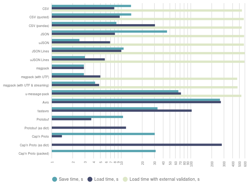
There are several conclusions which can be made by looking at that chart:
- Even basic validation implemented in pure Python will introduce a huge penalty for the execution time. Even the slowest SerDe with built-in basic validation will perform better.
- Official Avro implementation is incredibly slow. fastavro improves position of Avro, but it is still far beyond sane values.
- If you still trust Cap’n Proto and you do not need to convert its records into something else, you can try it, but I would not recommend it.
- Protobuf looks quite good among the others formats, which rely on data schema.
- msgpack looks like a very confident solution among schemaless formats. Speaking about its streaming mode, it can compete with uJSON Lines.
- It’s highly probable that CSV is not an option for you, until your client forces you to use it, so that data can be imported into Excel or similar spreadsheet-editing software.
The following figure depicts a chart with information about RAM consumed by different SerDe during deserialization.
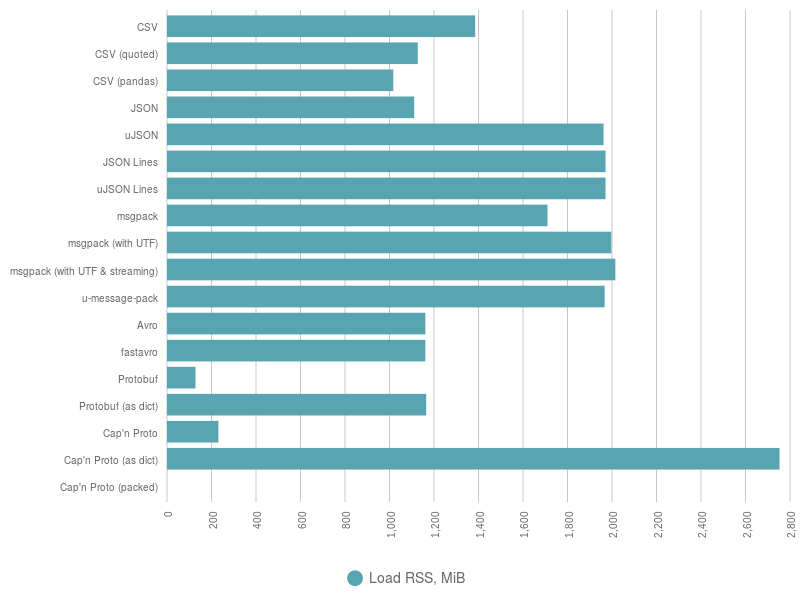
Note that to make an honest comparison of RAM consumption it’s better to take into consideration only cases which can be casted to a common factor, which is dict for us. Dicts in Python are heavy. It’s much cheaper to use namedtuple or a custom class with __slots__, but no schemaless libraries allow the use of custom output format for that, hence, dict is the only option.
From such perspective, three major groups can be clearly outlined:
- Not hungry: CSV, JSON, Avro, Protobuf.
- Hungry: uJSON, JSON Lines, uJSON Lines, msgpack.
- Monsters: Cap’n Proto.
Finally, a figure below displays a chart with information about disc space consumption by different SerDe, including different options.
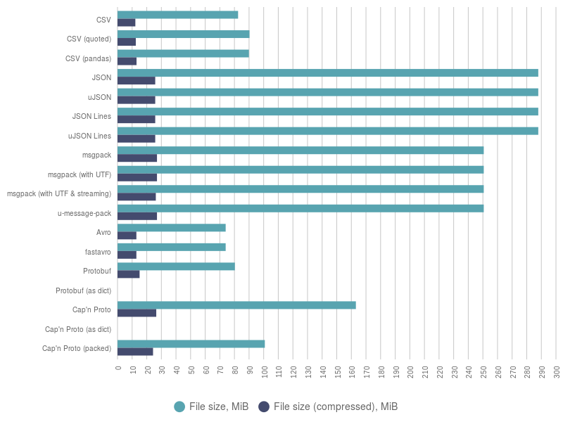
Here we can see that CSV, Avro, and Protobuf have the smallest raw and compressed file sizes.
Notably, JSON Lines, which uses an extra message delimiter, does not consume much more space than plain JSON. Their raw size is not much bigger than size of raw msgpack file. Compressed files are almost the same for these formats.
The size of Cap’n Proto files lays somewhere between the others. Remember that Cap’n Proto has a limit for size of data being deserialized. Also, a packed version of it can throw errors on you.
Conclusions
The main goal of this article was to observe and compare popular serialization formats and to reveal peculiarities of their usage in Python.
Note, that schema-dependent formats, such as Avro, Protobuf and Cap’n Proto, also provide own RPC facilities in addition to serialization and deserialization. These facilities were not observed in this article because they use own IPC clients and may rely on technologies, which are incompatible with the technological stack of your project. Please, refer to official documentation of those formats for details about their RPC facilities.
And now let’s recap several key points and draw a bottom line.
First of all, it’s clear that Cap’n Proto is an outsider among the formats observed. It has a horrible documentation for Python implementation, it’s buggy, it consumes too much time and memory when deserialized data is converted into dicts, it forces you to use field names in camel case, it does not provide support of empty values and so on. I believe it will be improved along with its documentation and someday it will find its place on the market. However, at this moment it doesn’t look ready for production.
Secondly, Avro looks not so bad, but it’s overwhelmingly slow.
CSV might be an option, but only if there’s no choice. It’s a text-centric format with a limited ability to store numeric data. If there’s a hard requirement to store data in format, which can be accessed via Excel and so on, then it can be better just to export needed data to CSV instead of keeping everything in it. By the way, applications like Excel have a limit for a number of records which can be stored in a single file. So, if your data set it very big (hundreds of thousands of records), you will need to split it into chunks, which means that you will end up with export procedure anyway.
Next, if your data is structured, then Protobuf can be your best friend. It is compact, fast, and supports schema evolution. It can look a bit clumsy and it does not provide streaming support, but even if you need to convert its deserialized records into dicts, it can still perform better than schemaless formats with custom validation.
Finally, JSON, JSON Lines and msgpack can offer speed and streaming support. One of them will be the best fit, depending on your needs and requirements. If data needs to be introspected by humans (e.g. HTTP API), then JSON will be fine. Otherwise, give msgpack a try.
As you can see, there’s no silver bullet and no definition of the most suitable SerDe—it depends on your needs and requirements. I hope this article helps you to make a wise choice. Feel free to share your experience and good luck!
This article originally appeared on Medium